Data
TOAST works with data organized into observations. Each observation is independent of any other observation. An observation consists of co-sampled detectors for some span of time. The intrinsic detector noise is assumed to be stationary within an observation. Typically there are other quantities which are constant for an observation (e.g. elevation, weather conditions, satellite procession axis, etc).
A TOAST workflow consists of one or more (distributed) observations representing the data, and a series of operators that “do stuff” with this data. The following sections detail the classes that represent TOAST data sets and how that data is distributed among many MPI processes.
Distribution
Although you can use TOAST without MPI, the package is designed for data that is distributed across many processes. When passing the data through a toast workflow, the data is divided up among processes based on the details of the toast.Comm class that is used and also the shape of the process grid in each observation.
A toast.Comm instance takes the global number of processes available (MPI.COMM_WORLD) and divides them into groups. Each process group is assigned one or more observations. Since observations are independent, this means that different groups can be independently working on separate observations in parallel. It also means that inter-process communication needed when working on a single observation can occur with a smaller set of processes.
-
class
toast.mpi.Comm(world=None, groupsize=0)[source]¶ Class which represents a two-level hierarchy of MPI communicators.
A Comm object splits the full set of processes into groups of size “group”. If group_size does not divide evenly into the size of the given communicator, then those processes remain idle.
A Comm object stores three MPI communicators: The “world” communicator given here, which contains all processes to consider, a “group” communicator (one per group), and a “rank” communicator which contains the processes with the same group-rank across all groups.
If MPI is not enabled, then all communicators are set to None.
Parameters: - world (mpi4py.MPI.Comm) – the MPI communicator containing all processes.
- group (int) – the size of each process group.
-
comm_group¶ The communicator shared by processes within this group.
-
comm_rank¶ The communicator shared by processes with the same group_rank.
-
comm_world¶ The world communicator.
-
group¶ The group containing this process.
-
group_rank¶ The rank of this process in the group communicator.
-
group_size¶ The size of the group containing this process.
-
ngroups¶ The number of process groups.
-
world_rank¶ The rank of this process in the world communicator.
-
world_size¶ The size of the world communicator.
Just to reiterate, if your toast.Comm has multiple process groups, then each group will have an independent list of observations in toast.Data.obs.
What about the data within an observation? A single observation is owned by exactly one of the process groups. The MPI communicator passed to the TOD constructor is the group communicator. Every process in the group will store some piece of the observation data. The division of data within an observation is controlled by the detranks option to the TOD constructor. This option defines the dimension of the rectangular “process grid” along the detector (as opposed to time) direction. Common values of detranks are:
- “1” (processes in the group have all detectors for some slice of time)
- Size of the group communicator (processes in the group have some of the detectors for the whole time range of the observation)
The detranks parameter must divide evenly into the number of processes in the group communicator.
Examples
It is useful to walk through the process of how data is distributed for a simple case. We have some number of observations in our data, and we also have some number of MPI processes in our world communicator:
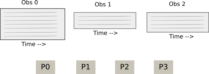
Starting point: Observations and MPI Processes.
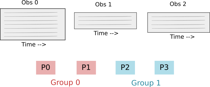
Defining the process groups: We divide the total processes into equal-sized groups.
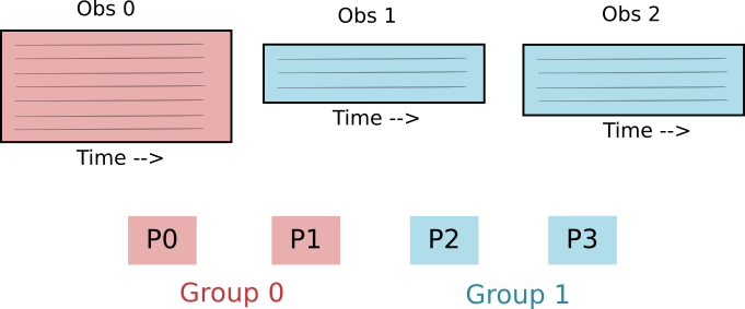
Assign observations to groups: Each observation is assigned to exactly one group. Each group has one or more observations.
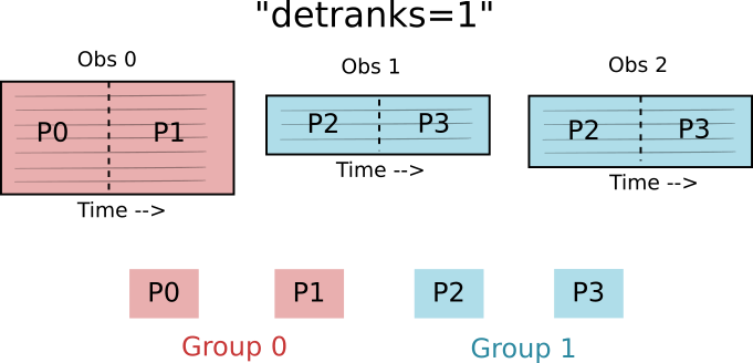
The detranks TOD constructor argument specifies how data within an observation is distributed among the processes in the group. The value sets the dimension of the process grid in the detector direction. In the above case, detranks = 1, so the process group is arranged in a one-dimensional grid in the time direction.

In the above case, the detranks parameter is set to the size of the group. This means that the process group is arranged in a one-dimensional grid in the process direction.
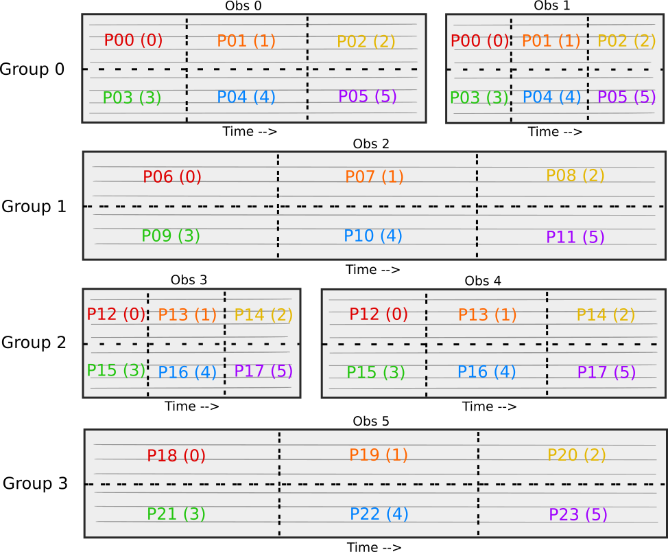
Now imagine a more complicated case (not currently used often if at all) where the process group is arranged in a two-dimensional grid. This is useful as a visualization exercise. Let’s say that MPI.COMM_WORLD has 24 processes. We split this into 4 groups of 6 procesess. There are 6 observations of varying lengths and every group has one or 2 observations. For this case, we are going to use detranks = 2. Here is a picture of what data each process would have. The global process number is shown as well as the rank within the group:
Built-in Data Support
In most cases of “real” experiments / telescopes, there will be custom TOAST classes to represent the data. However, TOAST comes with support for some (mainly simulated) data types. These are useful when simulating proposed experiments that do not yet have detailed specifications. Once a project reaches the level of having detailed hardware specifications (either designed or measured), then it should implement custom classes for that instrument description and data I/O or simulation.
Simulated TOD Classes
Recall that a TOD class represents the properties of some detectors from a telescope for one observation. This includes its physical location / motion through space as well as geometric locations of the detectors and (in the case of real data) methods to read detector data. For simulated TOD classes, we simulate the telescope boresight pointing and detector properties. We do not simulate detector data as part of the TOD class- that is done by various simulation operators that accumulate signal and noise from various sources. For generic satellite simulations, we have:
For generic ground-based simulations we have:
Simulated Noise Properties
One common noise model that is frequency used in simulations is a 1/f spectrum with white noise.
-
class
toast.tod.AnalyticNoise(*, detectors, rate, fmin, fknee, alpha, NET, indices=None)[source]¶ Class representing an analytic noise model.
This generates an analytic PSD for a set of detectors, given input values for the knee frequency, NET, exponent, sample rate, minimum frequency, etc.
Parameters: - detectors (list) – List of detectors.
- rate (dict) – Dictionary of sample rates in Hertz.
- fmin (dict) – Dictionary of minimum frequencies for high pass
- fknee (dict) – Dictionary of knee frequencies.
- alpha (dict) – Dictionary of alpha exponents (positive, not negative!).
- NET (dict) – Dictionary of detector NETs.
Simulated Intervals
Simulating regular data intervals is common task for many simulations:
-
toast.tod.regular_intervals(n, start, first, rate, duration, gap)[source]¶ Function to generate simulated regular intervals.
This creates a list of intervals, given a start time/sample and time span for the interval and the gap in time between intervals. The length of the interval and the total interval + gap are rounded down to the nearest sample and all intervals in the list are created using those lengths.
If the time span is an exact multiple of the sampling, then the final sample is excluded. The reason we always round down to the whole number of samples that fits inside the time range is so that the requested time span boundary (one hour, one day, etc) will fall in between the last sample of one interval and the first sample of the next.
Example: you want to simulate science observations of length 22 hours and then have 4 hours of down time (e.g. a cooler cycle). Specifying a duration of 22*3600 and a gap of 4*3600 will result in a total time for the science + gap of a fraction of a sample less than 26 hours. So the requested 26 hour mark will fall between the last sample of one regular interval and the first sample of the next. Note that this fraction of a sample will accumulate if you have many, many intervals.
This function is intended only for simulations- in the case of real data, the timestamp of every sample is known and boundaries between changes in the experimental configuration are already specified.
Parameters: - n (int) – the number of intervals.
- start (float) – the start time in seconds.
- first (int) – the first sample index, which occurs at “start”.
- rate (float) – the sample rate in Hz.
- duration (float) – the length of the interval in seconds.
- gap (float) – the length of the gap in seconds.
Returns: a list of Interval objects.
Return type: (list)